Global illumination is a phenomenon that helps render photo realistic images. Global illumination involves simulating both direct and indirect illumination. When light bounces off a surface once and is traced to the camera, we are simulating direct illumination.
However, light can bounce off several surfaces before reaching the camera. The color of a surface can be impacted by another object in the scene that bounced off light indirectly to it. This is called indirect illumination.
Without indirect illumination, some pixels may appear dark if they are not directly exposed to any of the light sources in the scene. However, they may not be completely dark in real as they may be exposed to light bounced off by other surfaces in the scene towards it. It may in fact be possible to observe color bleeding effects where the pixels may appear colored by diffuse reflections from other surfaces.
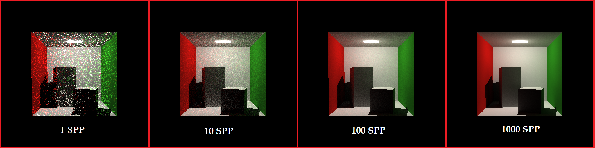
In this project, we use path tracing to simulate indirect diffuse reflections. Path tracing is a technique where many (10s to 1000s) reflected rays are traced at every point of intersection.
Consider a point P on a diffuse surface. Light that illuminates P can come from any direction in the hemisphere oriented about the normal at P. An ideal computation of the illumination at point P will require tracing an infinite number of rays across all directions in the hemisphere and adding their contributions. This is an integration problem.
As a more practical solution, the integral can be approximated using Monte Carlo Method. This involves sampling a fixed number of rays and averaging their contributions. The more the number of samples considered, the more accurate the computation will be. (It should be noted that there is a probability density function (PDF) in the Monte Carlo equation. This is to account for variance that can result from differing probabilities of picking the various samples. A sample that is more likely to be picked will unfairly contribute more to the average and hence has to be weighed down by its PDF factor).
To sample a ray in the hemisphere oriented about the normal at P, the following algorithm is used:
- Pick uniform random values for q1 and q2 in the [0,1] range.
- Assign polar coordinates Ө and Φ such that cosӨ = q1 and Φ = 2*𝜋*q2
- Transform the polar coordinates to Cartesian coordinates to create a sampled direction
- Create a new Cartesian coordinate system by assign the normal at P as the upvector
- Transform the direction obtained in (iii) into the coordinate system of (iv) and trace the ray from the point of intersection
To calculate the contribution of the ray, we use the rendering equation:
Lo(ωo) = Le(ωo) + ∫Ω f(ωi,ωo) Li(ωi) (ωi⋅n) dωi
- Lo – light directed outward along direction ωo (light received by camera)
- ωo – the direction of the outgoing light (view direction)
- Le – light emitted
- ∫Ω…dωi – integral over Ω
- Ω – the unit hemisphere centered around nn containing all possible values for ωiωi
- f(ωi,ωo) – the Bidirectional Reflectance Distribution Function (BRDF), the proportion of light reflected from ωi to ωo
- ωi – the negative direction of the incoming light
- Li – light coming inward from direction ωi
- n – the surface normal
- ωi⋅n – the weakening factor of outward irradiance due to cos of the angle between the incoming light direction and the surface normal (Lambertian Cosine Law)
The Bidirectional Reflectance Distribution Function (BRDF) gives the ratio of the light directed along the view direction ωo to the total incoming incoming light along ωi for a given point. Since we are simulating indirect diffuse reflections only, the Lambertian BRDF equation is considered:
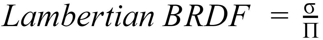
σ (albedo) is the diffuse reflectivity of the surface. Its value varies from 0 for a completely absorbing surface to 1 for a completely reflecting surface.
The integral in the Rendering Equation is approximated using Monte Carlo Equation.
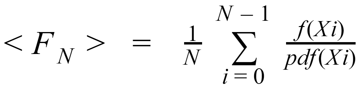
Since we are sampling uniformly, the PDFs of all the rays are the same and it can be proved that it is equal to 1/2𝜋
Hence the equation:
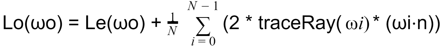
The recursive tracing of rays is terminated based on a predefined depth factor or when the contributions decrease below a threshold value.
Notes:
- While we use path tracing to cast multiple indirect diffuse reflected rays, we continue to cast a single specularly reflected and transmitted ray at every point of intersection as was done in Ray Tracing. This is done in order to optimize for rendering time.
- Phong Shading is used to compute direct illumination.
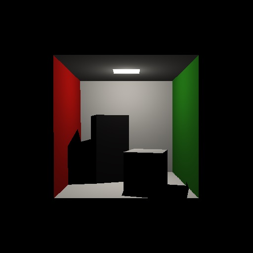
No Global Illumination 
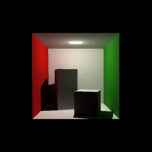
With Global Illuminations & 100 spp
Global Illumination with Area Lights
To account for area light sources for global illumination, they were considered like any other geometry with high emissive values. The emissive component was accounted in the first term of the rendering equation shown above.
Smaller Area Light 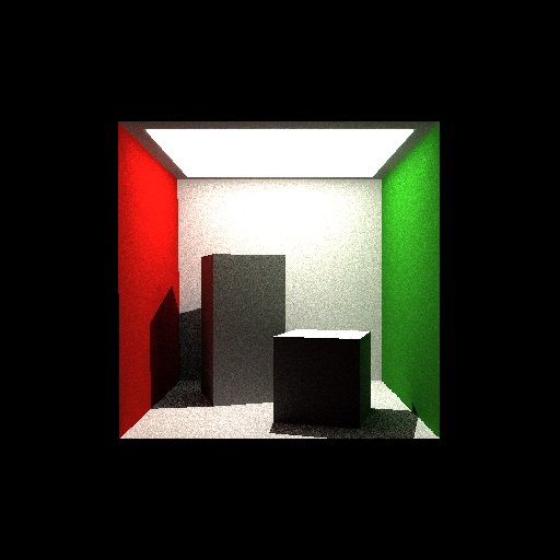
Larger Area Light
Importance Sampling
Apart from increasing the number of samples, using a better sampling technique can also help reduce noise. When we do uniform sampling, many of the samples chosen may be wasted in areas that make low contribution to the overall illumination of the point in consideration. For diffuse reflections, these can be directions that have a low Lambertian cosine factor. We can converge to the ideal value faster if we preferentially choose directions that have a higher cosine factor. Best results can be obtained if the sampling function also follows a cosine distribution. This is called as importance sampling.
As explained by Thomas Poulet, a cosine distribution can be achieved by selecting q1 = pow(rand(0,1), 0.5). We observed a minor decrease in noise by applying cosine sampling over uniform sampling.
