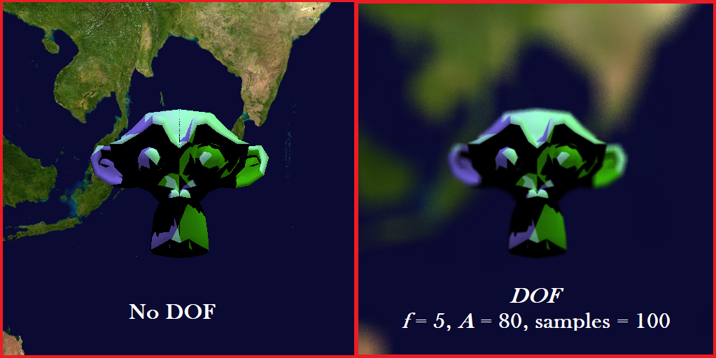
In ray tracer, we think of a pinhole camera model where all light is focused through an infinitesimally small point and onto the image plane. To add depth of field (DOF) effects, we simply have to replace this point camera with a lens.
Implementing depth of field in stochastic ray tracing consists of two parameters that influence out final image:
- Focal Length – determines how far objects must be from the camera to be in focus. Items closer than the focal point will be blurry, as will items farther away.
- Aperture – determines how blurry objects that are out of focus will appear. It defines the range of area around the focal point where objects appear mostly focused. In the limit case with an aperture size equal to zero, we are back to a pinhole camera where everything in the image is in focus.
Explanation
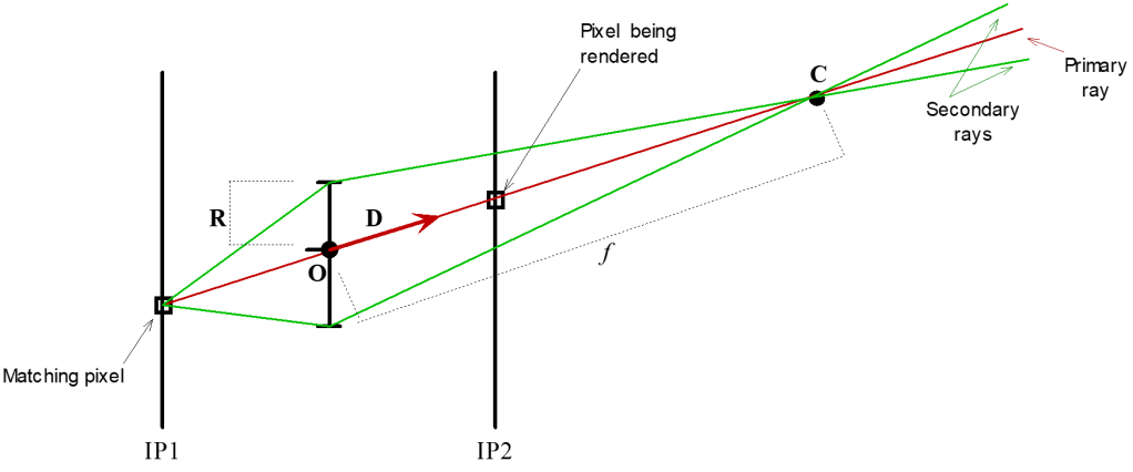
In the figure above, IP1 is the plane of the camera and IP2 is the image plane.We define the primary ray as we do in the ray tracer, i.e., O +tD
To get the convergence (C), we evaluate this with the focal length as C = O + fD
All rays for this pixel,primary and secondary, have to cross at the focal point. So this gives us a ray destination. Now we need to select some random point on the lens that a secondary ray will pass through. So, for some random small vector r that lies within our lens (limited by the aperture), we find a point (O + r) with direction C – (O + r) which forms our secondary ray.
Implementation Details
- Calculate the convergence point C using ray.origin (O), ray.direction (D), and focal length (f) as seen in the explanation before.
- To get the the blur effect, we shift the ray.origin (O) using the aperture variable and a random number generator.
- Now we recalculate the new ray direction for the shifted point as C – (O + r)
- We shoot multiple such secondary rays and average them for a pixel.
We can cast as many secondary rays as we want for a pixel, and the more we sample the better the image will look.
Variation in Focal Length (f)
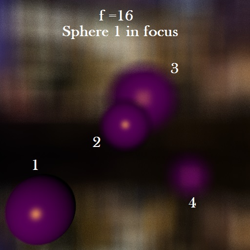
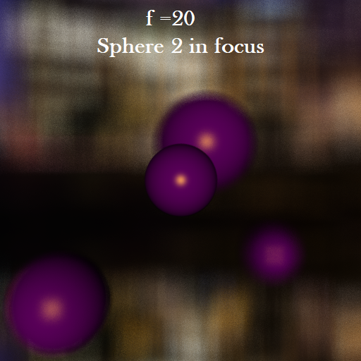

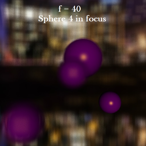
All the images above are rendered with 200 samples per pixel and an aperture of 500.
Variation in Aperture (A)
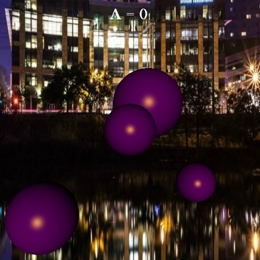
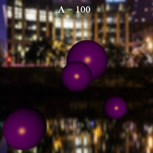

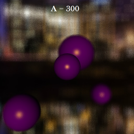

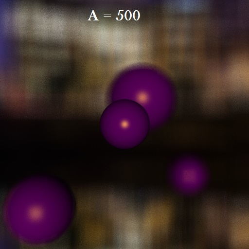
All the images above are rendered with 200 samples per pixel and an focal length of 20 so as to focus on Sphere 2 (middle one). As mentioned earlier, for A = 0, we have everything in focus as we would have for a pinhole camera.
Sources: [1] https://courses.cs.washington.edu/courses/csep557/99au/projects/trace/depthoffield.doc
[2] https://medium.com/@elope139/depth-of-field-in-path-tracing-e61180417027
