Bump mapping is a technique in computer graphics for simulating bumps and wrinkles on the surface of an object. This is achieved by perturbing the surface normals of the object and using the perturbed normal during lighting calculations. The result is an apparently bumpy surface rather than a smooth surface although the surface of the underlying object is not changed. Bump mapping was introduced by James Blinn in 1978.
In bump mapping, unlike displacement mapping, the surface geometry is not modified. Instead only the surface normal is modified as if the surface had been displaced. The modified surface normal is then used for lighting calculations (using the Phong shading model) giving the appearance of detail instead of a smooth surface. Bump mapping is much faster and consumes less resources for the same level of detail compared to displacement mapping because the geometry remains unchanged.
Implementation Details
We use a height/bump map (like the image shown at the end) for simulating the surface displacement yielding the modified normal as shown by Blinn. So, a bump map is a texture that has displacements of the surface stored in it. The actual height of the displacements will depend on how we use the bump map (only the range [0,1] is stored there). In the lighting calculations we use this perturbed normal. The perturbation to add to the normal is the first derivative of the bump map and can be calculated as the following,
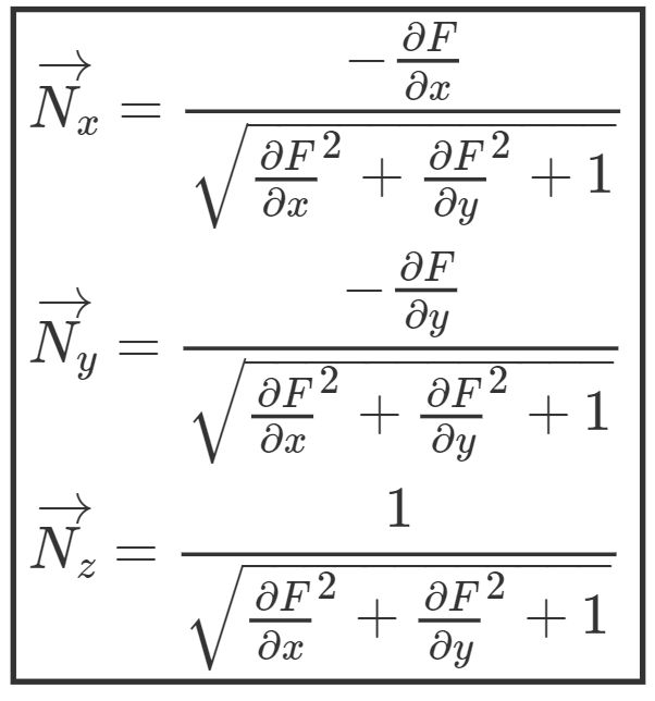
N reflects the changes stored in the bump map. In order to calculate the partial derivatives mentioned in the formula, the finite difference method is used. Finite difference is just taking a difference between two samples close enough together. For instance, finding the partial derivative of F with respect to x can be calculated with h = 1 and this gives us,
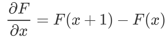
We do this for the a 2-D function such as F(u,v) in which case, the derivative w.r.t u is F(u+1,v) – F(u,v) and the derivative w.r.t. v is F(u,v+1) – F(u,v).
Before a lighting calculation is performed for each pixel on the object’s surface, the algorithm performs the following steps:
- Look up the height in the heightmap that corresponds to the position on the surface.
- Calculate the surface normal of the heightmap using the finite difference method as discussed above.
- Combine the surface normal from step two with the true (“geometric”) surface normal so that the combined normal points in a new direction.
- Calculate the interaction of the new “bumpy” surface with lights in the scene using the Phong reflection model.
The result is a surface that appears to have real depth. The algorithm also ensures that the surface appearance changes as lights in the scene are moved around. As it can be noticed from the algorithm, the surface itself is still flat, this method will only affect the lighting calculations and not the actual geometry.
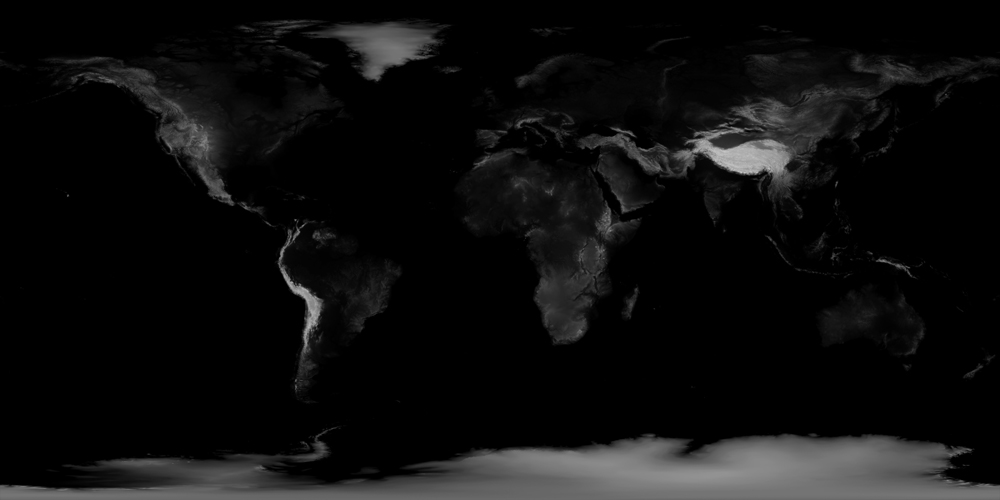
Bump Map 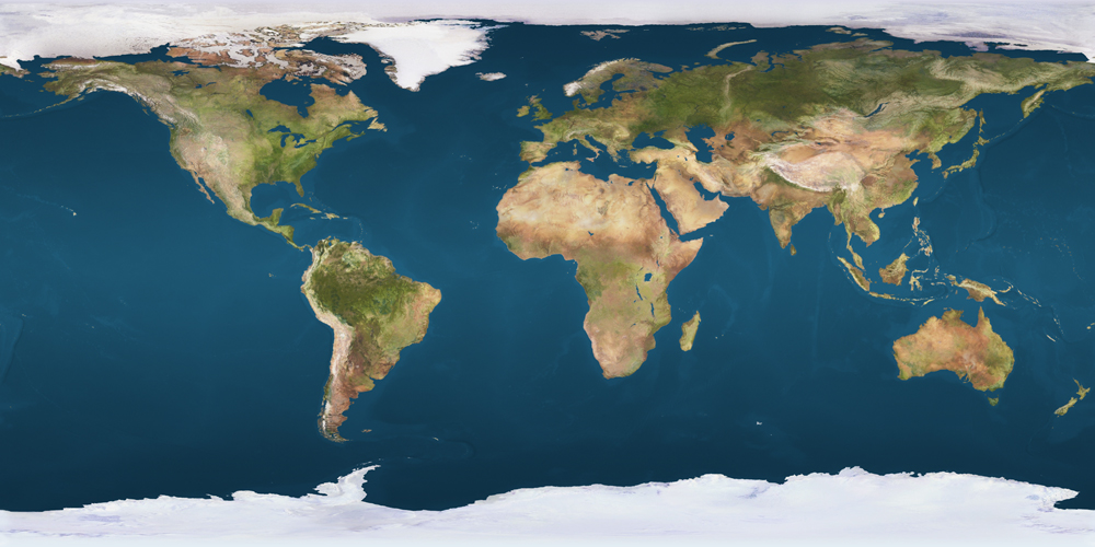
Texture Map 
Rendered Image with Texture Map + Bump Map
Variation with Bump Scale
We also provide the option of a “bump scale” that decides the degree of perturbation of the normals. A higher bump scale perturbs the normal more, causing the depressions to look more prominent.

Bump Scale = 5 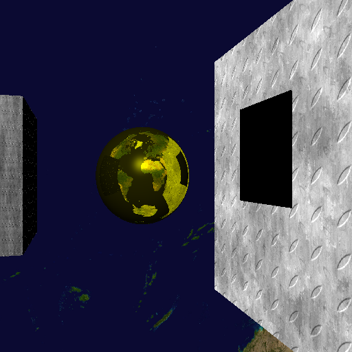
Bump Scale = 10 
Bump Scale = 30
